
PSTH significance#
PSTH significance tests a PSTH at every timepoint in its window, marking the stretches where the response differs from baseline, or from another event’s response. Testing every timepoint means the window of interest does not have to be chosen in advance.
Two kinds of comparison are computed:
Against zero. Is this event’s response different from baseline? Computed for every event automatically.
Between two events. Is the response to event A different from the response to event B? Computed for the event pairs named in the parameter form.
The bootstrap#
The figures in this section and the next are drawn from one example session, a single recording site with eighteen trials.
At each timepoint, GuPPy computes a confidence interval on the mean across trials — or, for a comparison between two events, on the difference between the two means. Timepoints whose interval excludes zero are candidates for significance.
The interval is built by resampling rather than from a formula:
Draw a resample of n trials, with replacement, from the n real trials. The resample is always the same size as the original, so some trials appear more than once and others not at all.
Average them into one synthetic mean waveform.
Repeat — 1000 times by default, set by Bootstrap Resamples.
At each timepoint there are now 1000 resampled means, one per repeat. Sorted, they form a distribution, and the interval’s lower and upper bounds are two percentiles of it.
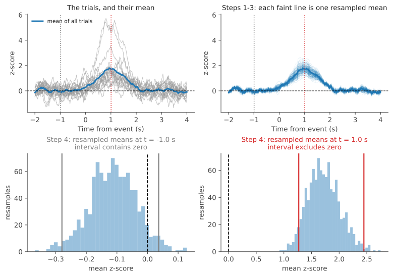
The bottom row is where the test happens. At the baseline timepoint the resampled means straddle zero and the interval contains it, so that timepoint is not significant. At the peak they sit well clear of zero and the interval excludes it, so it is. This significance check is repeated for every timepoint, generating a time series of significance values.
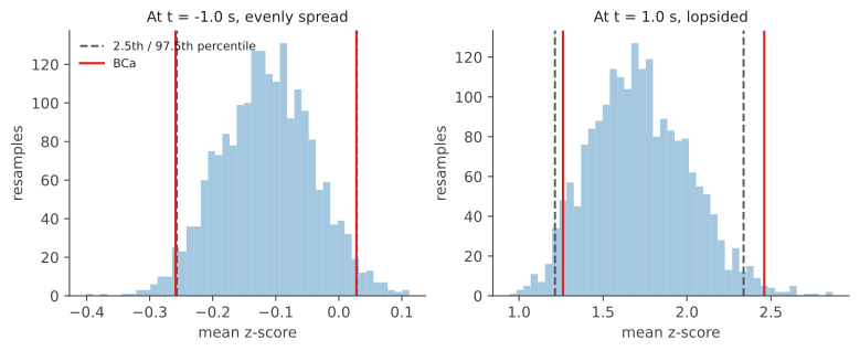
Step 4 above leaves open which two percentiles to take. For a 95% interval the naive answer is the 2.5th and the 97.5th. That is the right answer only if the distribution of resampled means is centered on the observed mean and equally spread either side of it, and photometry data often satisfies neither condition.
GuPPy takes the bias-corrected and accelerated (BCa) percentiles instead of the plain 2.5th and 97.5th. The name is just the two corrections it makes:
Bias correction handles a distribution that is off-center. If the resampled means do not fall half above and half below the observed mean, this measures how lopsided they are and moves both percentiles in that direction.
Acceleration handles a spread that is not constant. How wide the resampling distribution comes out often depends on the value of the mean itself — a larger response tends to be a more variable one — and this measures how quickly the width changes with the mean and adjusts the percentiles to match.
Both corrections are zero when the distribution is centered and evenly spread, which is why the two sets of bounds sit on top of each other in the left panel below. The more lopsided it is, the further they move. The interval’s coverage is set by Significance Level (alpha), so the default 0.05 asks for 95%.
Minimum duration#
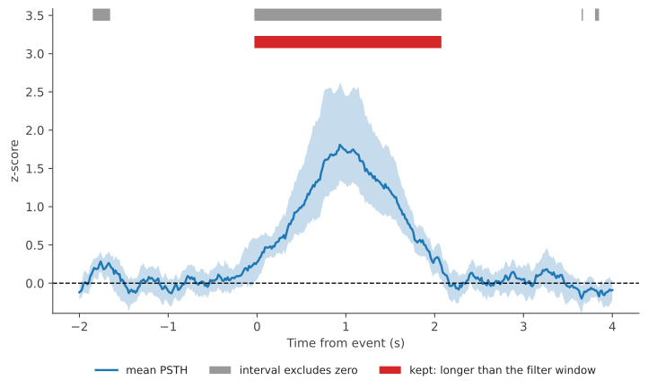
Because each timepoint’s interval is computed on its own, and because a PSTH window holds several thousand timepoints, some of them will clear zero by chance even when there is no real response to find. This is the multiple-comparisons problem, spread along the time axis. Those chance hits do not cluster in time, though: they land at scattered single timepoints, whereas a real response holds the interval clear of zero across a whole stretch of neighboring ones.
GuPPy separates them by duration, using a rule of thumb: consecutive significant timepoints form a run, and a run is kept only if it is longer than twice the moving-average filter window set in Step 3.
The threshold is twice the window because a run that long is the most that one or two chance deviations can produce between them. A moving average over N samples spreads each input sample across N output samples, so a single chance deviation comes out N samples wide, and two of them landing within N of each other merge into a run of at most 2N. Going beyond 2N takes three or more chance deviations falling in the right places at once, so a longer run is taken to come from the signal instead.
This is what controls the many comparisons. Instead of tightening the threshold each individual test has to clear, it requires neighboring tests to agree with each other, which chance hits do not do.
A filter window of zero leaves no shortest feature to compare against, which is why the significance test requires a non-zero one.
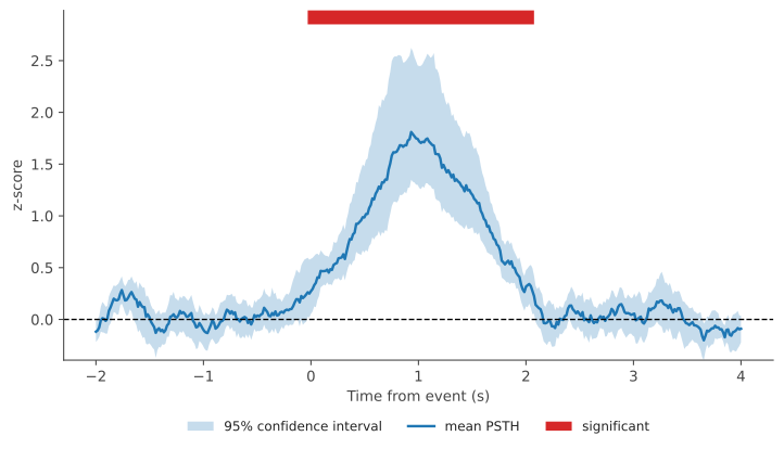
The Significance tab in Step 5 plots all of this together: the mean PSTH, its confidence interval, and a bar over the stretches where the interval excluded zero for longer than the duration threshold.
Group analysis#
Everything above describes a single session. The trials being resampled are that session’s trials, and the interval they produce is a statement about that session.
A group asks a broader question: not what happened in one recording, but what holds across a set of them. Photometry data is nested — trials sit inside a session, and sessions sit inside a group — and by the time a group reaches the significance test, Group Analysis has already reduced each of its sessions to one average response per event. Those session averages are what the bootstrap resamples, so the interval it produces describes the group.
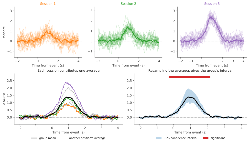
Summarizing each level of the hierarchy before moving up to the next is the standard treatment for nested data, and in many circumstances it is sufficient on its own. It is what makes the result a claim about the group rather than about the particular trials that happened to be recorded.
Trials from one session are not independent observations of the wider population; they resemble each other more than they resemble trials from another session. Analyzing them as though they were independent — pooling every trial from every session into a single sample — inflates the rate of false positives. See Further reading for the paper behind both points.
A comparison across a group tests two events against each other, or one event against zero, using the sessions in that group. Comparing one group against another is not supported yet.
Limitations#
Sessions in a group are treated as independent. If several come from the same animal they are not, and the interval will be too narrow in the same way. GuPPy has no concept of a subject, so it cannot detect this.
A significant stretch does not pin down when the response started. The result says the effect lies somewhere in that stretch, not that it begins at its left edge. Reading a precise onset off a boundary is the most common way this kind of analysis is over-read.
A response shorter than the duration threshold is discarded. The threshold cannot tell a brief real response from a chance hit, so it removes both. A wider moving-average filter window raises the threshold and discards more.
The duration rule is not a calibrated false-positive rate. The 2N threshold covers what the moving-average filter can build out of unstructured noise. A real recording carries noise structure of its own on top of that, which can hold the interval clear of zero for longer.
Small samples give unreliable intervals. Below three trials or sessions the bootstrap cannot run and the comparison is skipped. Between three and five it runs but is driven by a handful of distinct resamples; GuPPy logs a warning, and the sample count is recorded in the output.
Some timepoints have no interval. Trials near the start or end of a recording have their PSTH windows padded, and artifact removal blanks stretches of others. Where too few trials overlap at a timepoint, no interval can be computed there and that timepoint is reported as not significant. GuPPy warns when this affects a large fraction of a window.
Outputs#
Each comparison is written as its own table under psth_significance_output/, giving the time axis, the estimate, both interval bounds, the significance flag, the alpha it was computed at, and the sample count. The bounds are kept alongside the flag so a reader can see how close a non-significant stretch came and how wide the interval is where the sample size is small.
See Outputs for the file layout and Parameters for the settings that control the test.
Further reading#
The bootstrap is computed by scipy.stats.bootstrap with method="BCa". Its documentation covers the method and its references in more detail.
On summarizing nested data: McNabb and Murayama (2021), Current Research in Neurobiology show that analyzing nested data as though the points were independent of one another — pooling — inflates Type I error. On the other hand, summarizing each level (ex. averaging) and analyzing the summaries is reliable, robust, and sufficiently powered in most circumstances.